What the quantile really is?

Publish date: 2019-08-23

Intro

For few years when I was practicing data science I've used quantiles a lot. I knew what it is and when one should use it. I knew mathematical definition and intuition around quantiles but if someone would ask me to implement it from scratch I wouldn't know how to do it right away.

So what is a quantile? It's a one of most commonly used descriptive statistic. It gives us aggregated information about sample's distribution. For example let's say we have data sample representing salary of employees of some company. Quantile can gives us answer on question "How much should I be paid to earn more then 90% of employees?". Let's assume we have a sample

S = \lbrace 140, 80, 70, 200, 100 \rbrace

How would you answer the question for this sample? Probably by sorting salaries

70, 80, 100, 140, 200

and the answer would be somewhere between $140$ and $200$ . But where?

A bit of maths

Formally if $X$ is random variable with distribution $P$ and $p \in \lbrack 0, 1 \rbrack$ , then p-quantile is value $x_p$ of X which satisfy the following two inequalities

P(X \le x_p) \ge p \\ P(X \ge x_p) \ge 1 - p

But in real-world (statistics) we often don't know the real form of CDF of given sample. More interesting question is "how quantile is calculated?". At first it might not be obvious how one can implement quantile calculation just by looking at those formulas.

How it's calculated?

Statistics gives us an estimator for calculating quantile. This estimator also use order statistics of a sample. General form of p-quantile estimator $\hat{Q}(p)$ which is used in statistical software is as follows

\hat{Q}(p) = (1 - \gamma(p))X_{(j)} + \gamma(p) X_{(j+1)}

where $X_{(j)}$ is j-th order statistics of sample $x$ , $0 \le \gamma(p) \le 1$ and

\frac{j - m}{n} \le p \le \frac{j - m - 1}{n}

where $n$ is sample size.

So this estimator is exactly the same as our intuition from the beginning. It is somewhere between j-th and (j+1)-th ordered elements.

But where exactly? As it turns out there is not a good answer. Obviously we need some kind of interpolation with property $Q(p) \ge Q(q)$ if $p \ge q$ . This interpolation is mainly needed for small samples. If in our case sample had size of $100$ then $0.90$ quantile would be 90-th sorted element of the sample but in our five elements sample we cannot give specific answer without interpolation. In paper Sample Quantiles in Statistical Packages by Rob T. Hyndman and Yanan Fan there is summary of nine methods of interpolation defined in various statistical software.

Here we focus only on one specific method - default method from R programming language, from function quantile - type = 7. In this case $j = \lfloor p(n - 1) + 1 \rfloor$ and function $\gamma(p)$ is of the form

\gamma(p) = p(n - 1) + 1 - \lfloor p(n - 1) + 1 \rfloor

Now we can calculate 0.90-quantile of our five-element salaries sample - $n = 5$ and $p = 0.9$ . As we thought the answer lay somewhere between $140$ and $200$ now it is confirmed by above formulas - $j = \lfloor 0.9 \cdot 4 + 1 \rfloor = \lfloor 4.6 \rfloor = 4$ . Furthermore $\gamma(0.9) = 4.6 - 4 = 0.6$ . Finally we can compute

\hat{Q}(0.9) = (1 - \gamma(0.9))X_{(4)} + \gamma(0.9)X_{(5)} = \\ (1-0.6) \cdot 140 + 0.6 \cdot 200 = 176.0

So using default R method for calculating quantile we should expected final result as $176$ .

quantile(x = c(70, 80, 100, 140, 200), probs = 0.90)

Figure 1 presents how function $\gamma(p)$ interpolates between sample points. One can observe that interpolation is linear between nodes. It seems like reasonable method of interpolation.

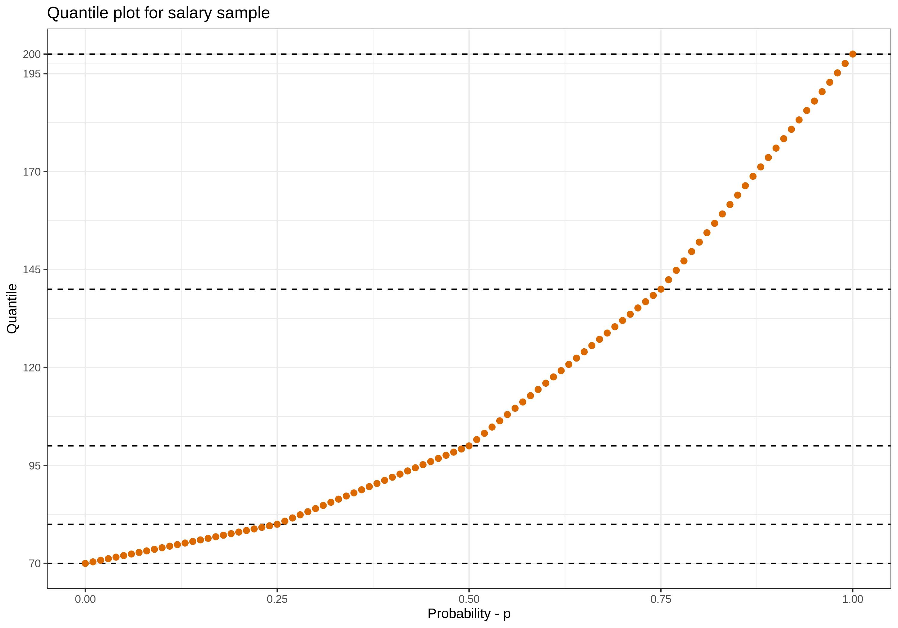
Figure 1: Quantile plot for salaries sample to present how interpolation looks like in this case.

Go implementation

Origin of this post came from little task I gave to myself - implementing in go bootstrap test for mean equality from paper An Introduction To The Bootstrap by Bradley Efron and Robert Tibshirani - revolutionary paper in modern statistics. For this implementation I've needed quantile. There is gonum library in go for mathematical and statistical functionalities where one can find implemented quantile function. At that point I asked myself a question "what the quantile really is?". I'm aware it's better to use already existing implementation but it was nice exercise, especially for someone with statistics or data science background.

So I've recreated quantile calculation in go with the same type of interpolation that is used as default type in R. It can be found here.

Summary

In my opinion quantile is one of most frequently used statistic from set of descriptive statistics. A sequence of quantiles of a sample gives us quality information about its distribution. I hope now, at the end of this post, you have an idea how this statistic is calculated in details. In particular it is worth to remember that calculated quantile value may doesn't exists in the sample. Also in sample with outlier (e.g. $\lbrace 0.5, 1.25, 5.32, 3.54, 1321.50 \rbrace$ ) p-quantiles for p close to $1.0$ would be artificial value. It's calculated as interpolation between one sample point and the outlier. In case when value of calculated quantile is "weird" now you know why.

If your software uses some external library to calculates quantiles make sure to know which type of interpolation this implementation is using. In some corner cases it might be helpful.